3D Gaussian Splatting made high-quality novel-view synthesis fast enough for interactive rendering. Its speed comes from an explicit scene representation: millions of 3D Gaussians, each carrying geometry, opacity, and appearance.
That representation is also the cost. More Gaussians mean more memory, storage, and data to transmit before a scene can be rendered somewhere else.
GaussianSpa starts from a different premise: simplification should be part of learning, not cleanup after learning.
Why pruning after training loses information
Each 3D Gaussian has a center, covariance, opacity, and spherical-harmonic coefficients. During rendering, the primitives are projected into the image plane and alpha-composited into pixels. This explicit structure makes rendering efficient, but scene size grows directly with the number of primitives.
Most simplification methods rank Gaussians with one signal — opacity, ray hit count, an importance score, or a learned mask — and remove a fixed fraction. Two problems follow.
First, one importance signal is incomplete. A primitive that appears unimportant globally may still carry a thin edge, a particular view, or a smooth background transition. Second, deletion is irreversible. Fine-tuning can adjust the survivors, but it cannot ask a removed Gaussian to hand off information it no longer has.
GaussianSpa delays that irreversible decision. The complete representation is allowed to adapt to the future budget before anything is permanently removed.
Make compactness an explicit constraint
Let $\mathbf{a}$ be the vector of Gaussian opacities, let $\Theta$ contain all other Gaussian parameters, and let $\mathcal{L}(\mathbf{a}, \Theta)$ be the standard reconstruction objective. GaussianSpa solves
\[\begin{aligned} \min_{\mathbf{a},\Theta} \quad & \mathcal{L}(\mathbf{a},\Theta) \\ \text{subject to} \quad & \lVert \mathbf{a} \rVert_0 \leq \kappa . \end{aligned}\]The $\ell_0$ constraint limits the number of nonzero opacities to the target budget $\kappa$. Because every Gaussian has one opacity and a zero-opacity Gaussian contributes nothing to the image, this is also a direct limit on the active Gaussian count.
The constraint says exactly what deployment needs: find the best-rendering scene that fits within a specified number of primitives. But $\ell_0$ sparsity is discrete and non-differentiable, so it cannot simply be inserted into ordinary gradient training.
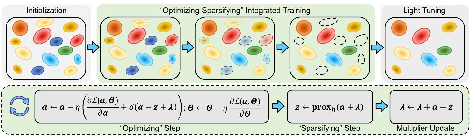
GaussianSpa introduces an auxiliary opacity vector $\mathbf{z}$ that is exactly sparse, then couples it to the trainable opacity vector $\mathbf{a}$ through an augmented Lagrangian. The original rendering problem and exact sparsity become separate, tractable updates.
The optimizing-sparsifying loop
Optimize the representation that will remain
The optimizing step continues to minimize rendering error while a quadratic penalty pulls the trainable opacity vector toward its exactly sparse counterpart:
\[\min_{\mathbf{a},\Theta} \mathcal{L}(\mathbf{a},\Theta) + \frac{\delta}{2} \left\lVert \mathbf{a}-\mathbf{z}+\lambda \right\rVert_2^2 .\]Position, scale, rotation, opacity, and appearance can all adapt. A Gaussian approaching zero still affects the gradients of the primitives that will survive, giving the representation time to transfer scene information.
Enforce the target count exactly
The sparsifying step projects $\mathbf{a}+\lambda$ onto the $\ell_0$ ball:
\[\mathbf{z} \leftarrow \operatorname{prox}_{h}\!\left(\mathbf{a}+\lambda\right), \qquad \lVert \mathbf{z} \rVert_0 \leq \kappa .\]Its solution is direct: keep the $\kappa$ largest elements and set the rest to zero. The projection acts on the auxiliary variable, so exact sparsity guides learning without deleting original primitives mid-transfer.
Delete only after convergence
The multiplier update $\lambda \leftarrow \lambda+\mathbf{a}-\mathbf{z}$ penalizes disagreement between the two opacity views. Over repeated updates, the distribution separates into near-zero and active groups. GaussianSpa starts this alternating process at iteration 15K, removes zero Gaussians at 25K, and finishes with light tuning.
This gradual schedule also explains the spatial pattern of the result: fewer, larger Gaussians can represent low-frequency sky or walls, while dense primitives remain around texture, contours, and fine geometry.
The quality-size trade-off
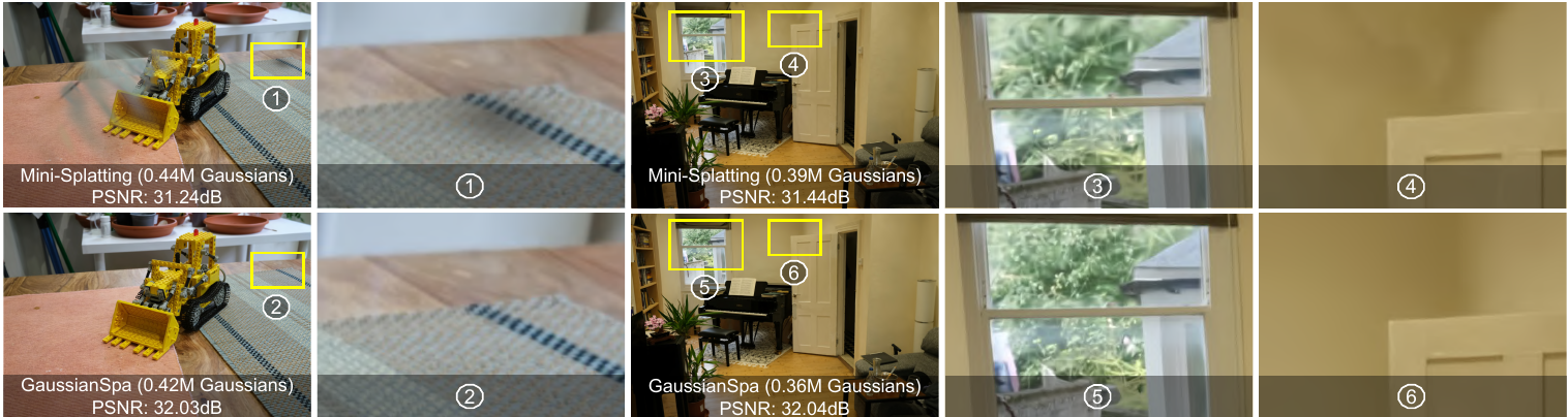
We evaluate GaussianSpa on Mip-NeRF 360, Tanks&Temples, and Deep Blending. Across all three datasets, the compact representation uses fewer Gaussians than Mini-Splatting while producing the highest PSNR in the comparison below.
Mip-NeRF 360
+0.40 dB PSNR
Tanks&Temples
+0.35 dB PSNR
Deep Blending
+0.91 dB PSNR
| Dataset | Method | PSNR ↑ | SSIM ↑ | LPIPS ↓ | #G (M) ↓ |
|---|---|---|---|---|---|
| Mip-NeRF 360 | 3DGS | 27.45 | 0.810 | 0.220 | 3.110 |
| Mini-Splatting | 27.40 | 0.821 | 0.219 | 0.559 | |
| GaussianSpa | 27.85 | 0.825 | 0.214 | 0.547 | |
| Tanks&Temples | 3DGS | 23.63 | 0.850 | 0.180 | 1.830 |
| Mini-Splatting | 23.45 | 0.841 | 0.186 | 0.319 | |
| GaussianSpa | 23.98 | 0.852 | 0.180 | 0.269 | |
| Deep Blending | 3DGS | 29.42 | 0.900 | 0.250 | 2.780 |
| Mini-Splatting | 30.05 | 0.909 | 0.254 | 0.397 | |
| GaussianSpa | 30.33 | 0.912 | 0.254 | 0.256 |
The qualitative and quantitative results tell the same story. Capacity is not removed uniformly. GaussianSpa preserves more primitives around high-frequency regions and lets broad, low-frequency areas use fewer, larger Gaussians.
Simplification and compression stack together
GaussianSpa reduces the primitive count; it does not need to redesign every attribute representation. Spherical-harmonic distillation, vector quantization, and other encoding techniques can be applied afterward.
When we add the compression operations used by LightGaussian, average Mip-NeRF 360 storage falls to 25 MB, compared with 42 MB for LightGaussian and 98 MB for EfficientGS.
| Method | PSNR ↑ | SSIM ↑ | LPIPS ↓ | Storage ↓ |
|---|---|---|---|---|
| EfficientGS | 27.38 | 0.817 | 0.216 | 98 MB |
| LightGaussian | 27.28 | 0.805 | 0.243 | 42 MB |
| GaussianSpa | 27.85 | 0.825 | 0.214 | 25 MB |
This modularity matters operationally. Simplification can be the first stage of a deployment pipeline rather than a competing alternative to quantization or attribute coding. The projection step can also adopt an existing importance criterion; the main contribution is the optimization framework around the criterion, not one handcrafted score.
Boundaries and open directions
GaussianSpa focuses on static 3DGS scenes and the quality-size trade-off. It does not yet solve every deployment constraint.
- The evaluation covers established novel-view synthesis datasets, not dynamic 4D scenes or city-scale reconstruction.
- Fewer Gaussians do not automatically minimize every byte or every millisecond; attributes still benefit from compression and runtime-aware encoding.
- The method introduces a target count, sparsity schedule, and penalty parameter that may need tuning for new scene families.
- PSNR, SSIM, and LPIPS measure rendering fidelity, not downstream geometric accuracy.
The constrained-optimization view can extend beyond primitive count — to spherical-harmonic order, precision, regional budgets, or dynamic representations where a primitive may matter only at certain times.
The bottom line
One-shot pruning asks which Gaussians look expendable now. GaussianSpa asks a more useful question: what is the best scene representation that can exist under this budget?
By making compactness part of training, separating differentiable rendering optimization from exact sparsity projection, and delaying deletion until information has migrated, GaussianSpa produces substantially smaller 3DGS models without accepting the usual quality penalty.
Citation
Please cite our original paper as:
@InProceedings{Zhang_2025_CVPR,
  author    = {Zhang, Yangming and Jia, Wenqi and Niu, Wei and Yin, Miao},
  title     = {GaussianSpa: An ''Optimizing-Sparsifying'' Simplification Framework for Compact and High-Quality 3D Gaussian Splatting},
  booktitle = {Proceedings of the IEEE/CVF Conference on Computer Vision and Pattern Recognition (CVPR)},
  month     = {June},
  year      = {2025},
  pages     = {26673-26682}
}